Wind Load on a Canopy
ASCE 7-16 added a new option to address wind loads on a canopy attached to a building with a h <= 60 ft [18.3 m]. This new criteria for canopies is addressed in ASCE 7-16 Section 30.11, and since it is in Section 30, the canopy is classified as Components and Cladding (C&C). The calculations are very straight forward and simple, and so we will show the calculation procedure and then show how the same calculation can be performed in the MecaWind software.
ASCE 7-16 Section 30.11: Attached Canopies on Buildings with h<= 60 ft [18.3 m]
In Chapter 30 Section 30.11 the ASCE 7-16 standard addresses the wind load on a canopy which is attached to a building. Table 30.11-1 outlines the steps we should follow:

Example:
Let’s work an example to illustrate this method of calculating the wind load on a canopy attached to a building.
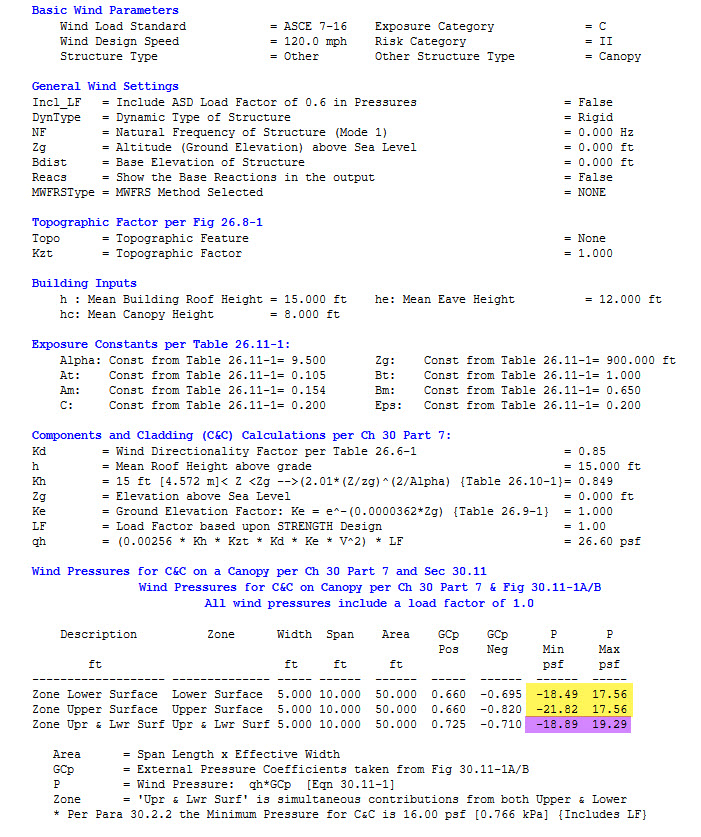
ASCE 7-16, 120 mph, Exp. C, Category II
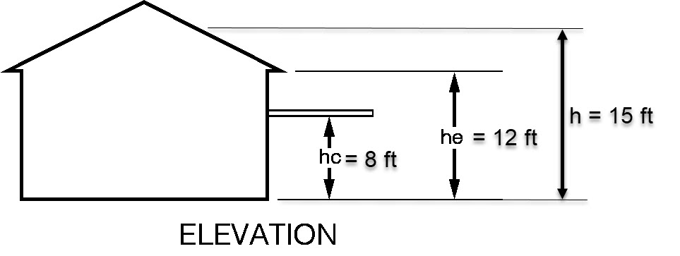
Mean Building Roof Height (h) = 15 ft
Mean Eave Height (he) = 12 ft
Mean Canopy Height (hc) = 8 ft
Table 26.11-1 for Exp C –> zmin = 15 ft, zg = 900 ft, Alpha = 9.5
z = 15 ft (Mean roof height)
Kh=2.01*(15 ft / 900 ft)^(2/9.5) = 0.849
Kzt = 1.0 (No topographic feature)
Kd = 0.85 (Building MWFRS per Table 26.6-1)
Ke = 1 (Sea Level)
Calculate Pressure at Mean Roof Height:
qh = 0.00256*Kh*Kzt*Kd*Ke*V^2
= 0.00256*0.849*1*0.85*1*120^2 = 26.6 psf
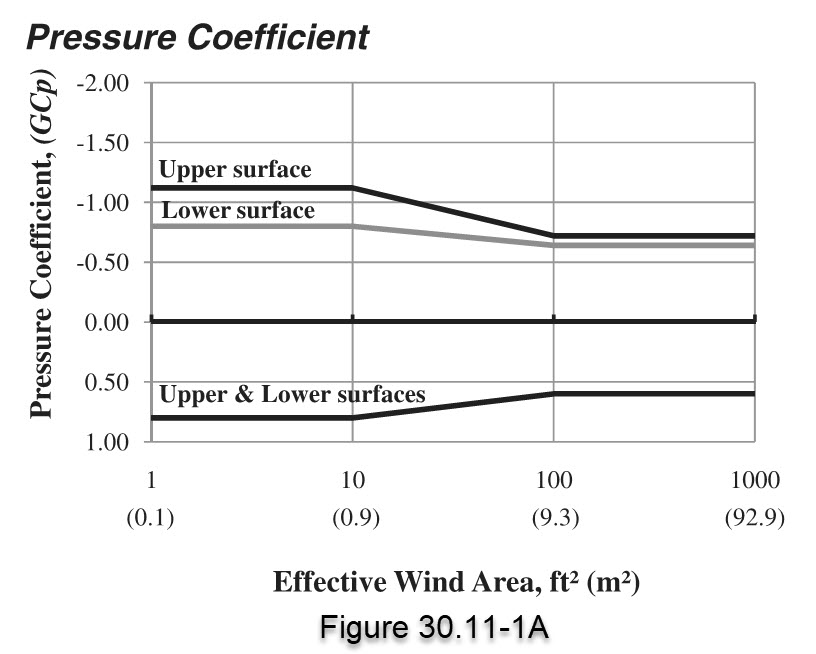
For the next part, we need the effective area in order to look up the GCp values from Figure 30.11-1A. If we don’t know the effective area, then the most conservative approach is to use an effective area of 10 sq ft [0.9 sq m] or less, since this yields the maximum values for GCp. In this case, our canopy is projecting 5 ft from wall, and 10 ft along the wall.
Effective wind area = 5 ft x 10 ft = 50 sq ft [4.64 sq m]
In Section 26.2, there is a definition for effective area that indicates that the width need not be less than 1/3 of the span length. In this section, Figure 30.11-1 is not mentioned, and so it is Meca’s interpretation that this rule must not apply to canopy design.
Consider upper and lower surfaces separately:
First we consider the case where the contribution from the upper and lower surfaces are considered separately. For this case, we look up the value of GCp using Figure 30.11-1A. As calculated previously, our effective area is 50 sq ft [4.64 sq m].
Lower Surface: GCp = -0.695 / +0.66
Upper Surface: GCp = -0.82 / +0.66
Lower Surface:
p = qh * GCp = 26.6 * -0.695 = -18.49 psf
= 26.6 * +0.66 = +17.56 psf
Upper Surface:
p = qh * GCp = 26.6 * -0.82 = -21.81 psf
= 26.6 * +0.66 = +17.56 psf
The convention in ASCE 7 is that positive (+) pressures are acting TOWARDS a surface and negative (-) pressures are acting AWAY from a surface.

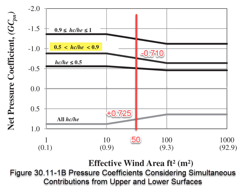
Combined net effect on upper and lower surfaces:
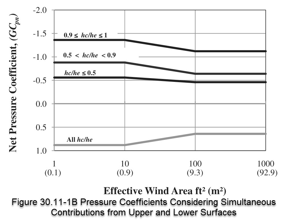
Now, let’s look at the case of the combined (net) effect of the pressures on the upper and lower surfaces. For this case, we look up the value of GCp using Figure 30.11-1B. As calculated previously, our effective area is 50 sq ft [4.64 sq m]. For this option, we also need to calculate the ratio hc/he in order to determine which curve to follow:
hc / he = 8 / 12 = 0.667
Upper and Lower Surface: GCp = -0.710 / +0.725
p = qh * GCp = 26.6 * -0.710 = -18.89 psf
= 26.6 * +0.725 = +19.29 psf
The convention in ASCE 7 is that positive (+) pressures are acting TOWARDS a surface and negative (-) pressures are acting AWAY from a surface.