How to Find Wind Pressure on Solar Panels

In this article we will investigate the procedure for calculating the design wind pressure on rooftop solar panels per ASCE 7-16 design code. I feel like the best way to describe this procedure is by working through an example, and that’s just what we will do. For this example, we will look at a 30ft tall building with a flat roof in Broken Arrow, Oklahoma.
Background:
The typical dimensions for a residential solar panel is 65″ long and 39″ wide.
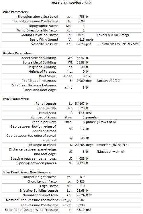
The design wind speed for zip code 74011 with exposure C and risk category III is 115.0 mph, and the elevation above sea level is 755 ft. We won’t go in depth in this article on the procedure for calculating the velocity pressure, but for h=30ft it comes out to be qh = 32.28 psf.
In ASCE 7-16 there are two sections that cover rooftop solar panels: 29.4.3 and 29.4.4. Section 29.4.3 addresses buildings of all heights with a flat roof or gable/hip roofs with a slight slope (less than 7 degrees). Section 29.4.4 covers the other roof slopes. Each have their own restrictions on the parameters that can be used due to wind tunnel testing done to develop the procedures and normal use of solar panel arrays. In this example we will focus on section 29.4.3, which utilizes figure 29.4-7.
Solar Panel Wind Pressure Parameters:
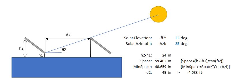
We will use the typical residential solar panel dimensions and we will do 3 rows of 8 panels in the array. The bottom edge of the panel will have a 1 ft gap between the roof surface and the top edge will have a 3ft gap, giving a tilt angle of 20.3 degs. The minimum horizontal clear distance between the panels and the edge of the roof is the larger of 2(h2-hpt) and 4ft. In our case, there is no parapet (hpt) and the clear distance comes out to be 6ft. The minimum gap between panels is 0.25 inches, but we will use a spacing of 1.5 inches in this example. For the spacing between each row (array) of solar panels, we want to optimize this so the rows aren’t in the shadow of the adjacent row. We will need to know the solar elevation and azimuth for our location, and this can be found using a Solar Chart Program from the University of Oregon, as seen below. We are going to use a time range of 10am to about 2:45pm in the Winter season.
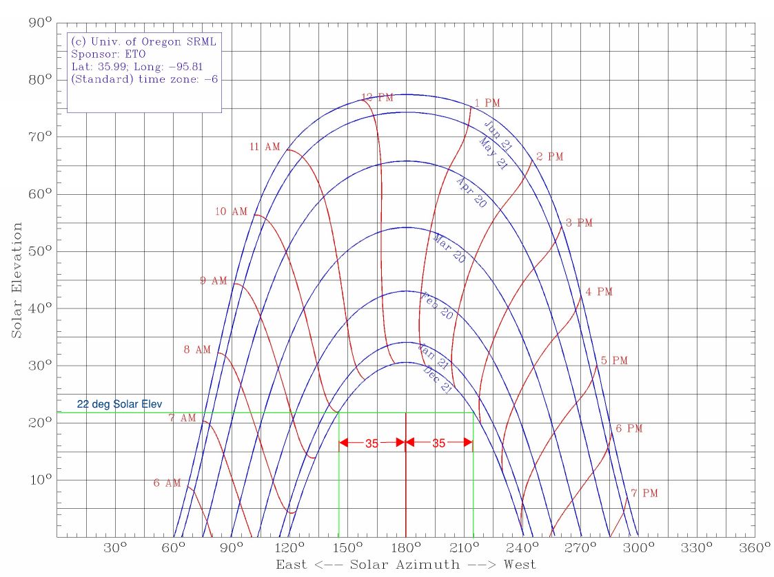
The chart shows a solar elevation of 22 degrees and an azimuth correction of 35 degrees. Now to find the spacing between the arrays we will divide the height difference of the panel edges by the tangent of the solar elevation, and then correct for the azimuth by multiplying this spacing by the cosine of the azimuth correction and rounding our answer up to the nearest whole inch. This process yields a spacing of 49 inches, and is illustrated below.
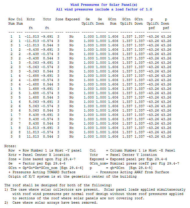
For the sake of this example, I am going to place the solar panels in the center of the building. Taking into account the panel edge to roof edge (d1=6ft), the spacing between rows (d2=4.083ft), and the spacing between panels (d3=0.125ft), the building width parallel to the solar array is 38.875ft (WL=38.875ft) and the building width perpendicular to the solar array is 36.416ft (WS=36.416ft).
Solar Panel Design Wind Pressure:
The equation we need to solve for the design wind pressure for rooftop solar panels is:

- yp: minimum of (1.2, 0.9+hpt/h)
- yc: maximum of (0.6+0.06*Lp, 0.8)
- yE: 1.5 for uplift loads on panels that are exposed and within a distance of 1.5*Lp from the end of a row at an exposed edge of an array
- yE: 1.0 elsewhere for uplift loads and for all downward loads, as illustrated in Fig. 29.4-7
A panel is defined as exposed if d1 to the roof edge > 0.5*h and at least one of the following applies:
- d1 to the adjacent array or roof edge > max (4*h2, 4ft)
- d2 to the next adjacent panel > max (4*h2, 4ft)
In our example, the d1 value is set as the minimum horizontal clear edge distance of 6ft, and the height of the building is 30ft. Evaluating the expression for an exposed panel shows that d1 (6ft) is not greater than 0.5*h (0.5*30=15ft), so all the panels will use yE = 1.0.
Now solving for our other gamma values:
yp = min(1.2, 0.9+hpt/h) = min(1.2, 0.9+0/30)
yp = 0.9
yc = max(0.6+0.06*Lp, 0.8) = max(0.6+0.06*5.4167ft, 0.8)
yc = 0.925
Utilizing ASCE 7-16 Fig. 29.4-7:
We will need to use Fig. 29.4-7 to find our GCrn,nom value to use in our solar panel design wind speed equation. For each solar panel, we will need to establish which zone it is in using the “Building Roof Plan” in the figure. In this example, our boundary for the edges is actually greater than either of the building widths (2*h=2*30=60 >WS and WL), thus every panel is in zone 3. The next thing we need is the “Normalized Wind Area” which is defined as:
- An = (1000/[max(Lb,15)^2])*A
– where A is the effective wind area of the solar panel (Lp*Wp) and Lb is the minimum of (0.4*(h*WL)^0.5, h, Ws) - Lb = (0.4*(30*38.875)^0.5, 30, 36.416)
Lb = 13.66 ft - An = (1000/[max(13.66,15)^2])*(5.4167*3.25)
An = 78.24 ft^2
Finally, to know which “Nominal Net Pressure Coefficient” graph to use, we need to know the tilt angle of our solar panels. This can be found by taking the inverse tangent of the height difference of the panel edges to the roof surface divided by the length of the panel (w=arctan[(h2-h1)/Lp]). Solving for the tilt angle we get 20.27 degrees (arctan[(3-1)/5.4167]), which means we will use the right GCrn,nom graph since it is between 15 and 35 degrees.

From inspection of this graph we see that the y-intercept is 3.5 and that the slope is -1 from An = [<1, 500]. This gives us an equation of the line as GCrn,nom = -log(An) + 3.5. Plugging in 78.24 ft^2 for An, GCrn,nom equates to 1.607.
Now we can equate GCrn and thus the solar panel design wind pressure, p:
GCrn = yp*yc*yE*GCrn,nom
GCrn = 0.9*0.925*1.0*1.607
GCrn = 1.338
p = qh*GCrn
p = 32.284*1.338
p = 43.191 psf
So with the parameters and location used in the example, each solar panel would see a design wind pressure of an uplift and downward load of +/- 43.191 psf. Every panel seeing the same wind pressure isn’t usually the case. If the panel is in a different zone than another, then the GCrn value will be different. If the panel is considered exposed, then the yE value will be different giving a different GCrn. So in those cases you would need to go back and redo the calculations for those panels.